The SHE equations incorporate material-specific properties by the velocity term $\mathbf v$ , the modulus $\vert \mathbf \mathbf k \vert$ of the wave vector as a function of energy, the generalized density of states , and the scattering operator . However, the velocity term $\mathbf v$ and the density of states are not independent and depend on the dispersion relation $\varepsilon(\mathbf k)$ by

$\begin{align*} \mathbf v &= \frac{1}{\hbar} \nabla_{\mathbf k} \varepsilon \ , \\ Z(\varepsilon, \theta, \varphi) &= \frac{\vert \mathbf k \vert^2}{4\pi^3} \frac{\partial \vert \mathbf k \vert}{\partial \varepsilon} \ . \end{align*}$

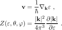
Note that different prefactors for the definition of the density of states are in use, thus extra care needs to be taken when comparing values for the density of states from different sources. The third quantity, namely the modulus of the wave vector, is obtained from inverting the dispersion relation. Consequently, the choice of the dispersion relation plays a central role for the accuracy of the SHE method. The dispersion relations available in ViennaSHE are discussed below.

The second half of this chapter is devoted to the various scattering effects. Since scattering balances the energy gain of carriers due to the electric field, accurate expressions for the scattering operators are mandatory. ViennaSHE provides the most important linear scattering operators, see Scattering Mechanisms

Warning: Keep in mind that ViennaSHE is not rigorously calibrated! Before any quantitative interpretation of the obtained simulation results, ensure a proper calibration for your application domain first.

Dispersion Relations

ViennaSHE includes three common dispersion relations used for the SHE method. All relations are spherically symmetric in the Herring-Vogt transformed space, which has been shown to be a fairly good approximation [7] [9].

Parabolic Dispersion

Due to the nonuniformity of the crystal lattice in silicon with respect to a change in direction, the dispersion relation linking the particle momentum with the particle energy cannot be accurately described by the idealized setting of an infinitely deep quantum well, for which the solution of Schrödinger's equation yields a parabolic dependence of the energy on the wave vector:

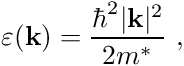
$\begin{align*} \varepsilon(\mathbf{k}) = \frac{\hbar^2 \vert\mathbf{k}\vert^2}{2 m^* } \ , \end{align*}$

where $\hbar$ is the scaled Planck constant and is the effective mass. Still, this quadratic relationship termed parabolic band approximation is a good approximation near the minimum of the energy valley. Due to its simple analytical form, the parabolic dispersion relation is often used up to high energies, for which it fails to provide an accurate description of the material.

Non-Parabolic Dispersion (Modena)

A more accurate approximation to the band structure in silicon can be obtained by a slight modification of the form

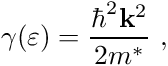
$\begin{align*} \gamma(\varepsilon) = \frac{\hbar^2 \mathbf{k}^2}{2 m^* } \ , \end{align*}$

where the typical choice

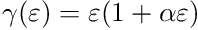
$\begin{align*} \gamma(\varepsilon) = \varepsilon ( 1 + \alpha \varepsilon) \end{align*}$

is known as Kane's model [13]. The parameter $\alpha$ is called nonparabolicity factor; in the case $\alpha = 0$ one obtains again the parabolic dispersion relation. The non-parabolic approximation with $\alpha = 0.5$ already provides a good approximation of the dispersion relation for electrons in relaxed silicon at low energies. However, for kinetic energies above eV the nonparabolic approximation fails to describe the nonmonotonicity of the density of states in silicon.

The non-parabolic dispersion relation is usually referred to as Modena model in publications on the SHE method [6] [9], thus ViennaSHE follows this nomenclature.

Extended Vecchi Model

Without going into the details of the derivation, it is possible to drop the assumption of having an explicit dispersion relation $\varepsilon(\mathbf k)$ , and instead use fullband-data for the velocity and the density of states directly. This model proposed by Jin et al. [9] is referred to as extended Vecchi model, as a similar idea restricted to first-order SHE has been used by Vecchi et al. [25].

To summarize, an overview of different dispersion relations is as follows:

Comparison of the density of states and the carrier velocity for the various band models. The many-band model [2] and the fitted full-band model from Matz et al. [17] are not included in ViennaSHE as they are superseded by the fullband-model of Jin et al. [9]

Scattering Mechanisms

While the band structure links the particle energy with the particle momentum, it does not fully describe the propagation of carriers. In the presence of an electrostatic force, carriers would be accelerated and thus gain energy indefinitely unless scattering with the crystal lattice or with other carriers is included in the model. ViennaSHE provides the most important scattering mechanisms in relaxed silicon, which are discussed in the following. The scattering operator is assumed to be given in the form

$\begin{align*} Q\{f\} = \frac{1}{(2\pi)^3} \int_{\mathcal{BZ}} s(\mathbf{x}, \mathbf{k}^\prime, \mathbf{k}) f(\mathbf{x}, \mathbf{k}^\prime, t) - s(\mathbf{x}, \mathbf{k}, \mathbf{k}^\prime) f(\mathbf{x}, \mathbf{k}, t) \: \mathrm{d}\mathbf k^\prime \ , \end{align*}$

where it has to emphasized that scaling factors in front of the scattering integral, here $1/(2\pi)^3$ , need to be taken into account when comparing scattering rates from different sources. The commonly written small sample volume $V_{\mathrm s}$ as prefactor for the scattering integral is not written explicitly in the following.

A detailed discussion of scattering mechanisms can be found e.g.~in the book of Lundstrom [14] . In the context of the SHE method, various scattering mechanisms are discussed by Hong et al. [7].

Acoustical Phonon Scattering

Atoms in the crystal lattice vibrate around their fixed equilibrium locations at nonzero temperature. These vibrations are quantized by phonons with energy $\hbar \omega_{\mathrm{phon}}$ . Since the change in particle energy due to acoustic phonon scattering is very small, the process is typically modelled as an elastic process. The scattering rate can thus be written as

$\begin{align*} s_{\mathrm{ac}}(\mathbf{x}, \mathbf{k}, \mathbf{k}^\prime) = \sigma_{\mathrm{ac}} \delta(\varepsilon(\mathbf{k}) - \varepsilon(\mathbf{k}^\prime)) \ , \end{align*}$

where the coefficient $\sigma_{\mathrm{ac}}$ is given by

$\begin{align*} \sigma_{\mathrm{ac}} = \frac{2 \pi k_{\mathrm{B}}T \mathcal{E}^2}{\hbar \rho u_{\mathrm l}^2 } \ , \end{align*}$

with deformation potential $\mathcal E$ , density of mass $\rho$ , and longitudinal sound velocity $u_{\mathrm l}$ .

	Si	Ge
$\rho$	g/cm	5.32 g/cm
$u_{\mathrm l}$	$9.05 \times 10^5$ cm/s	$5.40 \times 10^5$ cm/s
$\epsilon$	$11.7 \times \epsilon_0$	$16.0 \times \epsilon_0$
$\mathcal E_{\mathrm e}$	eV	eV
$\mathcal E_{\mathrm h}$	eV	eV

Material parameters for silicon and germanium, cf. [11].
The subscripts $\mathrm e$ and $\mathrm h$ are used to distinguish between electrons and holes.

Since acoustic phonon scattering is modeled as an elastic scattering process [8], it does not couple different energy levels.

Optical Phonon Scattering

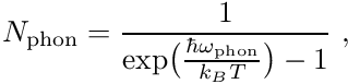
Unlike acoustical phonon scattering, optical phonon scattering is modelled as an inelastic process leading to a change of the particle energy. With the phonon occupation number $N_{\mathrm{phon}}$ given by the Bose-Einstein statistics

$\begin{align*} N_{\mathrm{phon}} = \frac{1}{\exp\bigl(\frac{\hbar \omega_{\mathrm{phon}}}{k_B T}\bigr) - 1} \ , \end{align*}$

the scattering rate for the initial state $\mathbf{k}$ and the final state $\mathbf{k}^\prime$ can be written as

$\begin{align*} s_{\mathrm{op}}(\mathbf{x}, \mathbf{k}, \mathbf{k}^\prime) = \sigma_{\mathrm{op}} \bigl[ N_{\mathrm{phon}}\hphantom{)} \delta(\varepsilon(\mathbf{k}) - \varepsilon(\mathbf{k}^\prime) + \hbar \omega_{\mathrm{op}}) + (1+N_{\mathrm{phon}}) \delta(\varepsilon(\mathbf{k}) - \varepsilon(\mathbf{k}^\prime) - \hbar \omega_{\mathrm{op}}) \bigr] \ , \end{align*}$

where $\sigma_{\mathrm{op}} (\mathbf{x}, \mathbf{k}, \mathbf{k}^\prime)$ is symmetric in $\mathbf{k}$ and $\mathbf{k}^\prime$ and given by

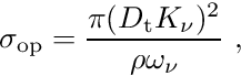
$\begin{align*} \sigma_{\mathrm{op}} = \frac{\pi (D_{\mathrm t} K_\nu)^2}{\rho \omega_\nu} \ , \end{align*}$

with coupling constant $D_{\mathrm t} K_\nu$ , mass density $\rho$ , and phonon frequency $\omega_\nu$ . Values for the individual modes are as follows:

$D_{\mathrm t} K$	$4.0 \times 10^8$ eV/cm
$\hbar \omega_{\mathrm op}$	meV

Parameters used for optical phonon scattering in ViennaSHE as published in [12] .

It should be noted that optical phonon scattering couples the energy levels $H - \hbar \omega_{\mathrm{op}}$ , and $H + \hbar \omega_{\mathrm{op}}$ in an asymmetric manner, because scattering from higher energy to lower energy is more likely than vice versa.

Ionized Impurity Scattering

Dopants in a semiconductor are fixed charges inside the crystal lattice. Since carriers are charged particles as well, their trajectories are influenced by these fixed charges, leading to a change of their momentum. The model by Brooks and Herring [1] [8] suggests an elastic scattering process with scattering coefficient

$\begin{align*} s_{\mathrm{imp}}(\mathbf{x}, \mathbf{k}, \mathbf{k}^\prime) = \sigma_{\mathrm{imp}}(\mathbf{x}, \mathbf{k}, \mathbf{k}^\prime) \delta(\varepsilon(\mathbf{x}) - \varepsilon(\mathbf{x}^\prime)) \ , \end{align*}$

where $\sigma_{\mathrm{imp}} (\mathbf{x}, \mathbf{k}, \mathbf{k}^\prime)$ is symmetric in $\mathbf{k}$ and $\mathbf{k}^\prime$ and given by

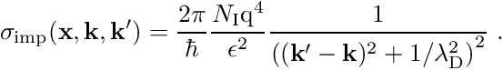
$\begin{align*} \sigma_{\mathrm{imp}}(\mathbf{x}, \mathbf{k}, \mathbf{k}^\prime) = \frac{2\pi}{\hbar} \frac{N_{\mathrm I} \mathrm{q}^4}{\epsilon^2} \frac{1}{\left( (\mathbf k^\prime - \mathbf k)^2 + 1/\lambda_{\mathrm D}^2 \right)^2} \ . \end{align*}$

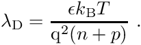
The ordinality of the impurity charge is assumed to be one, and $N_{\mathrm a}$ and $N_{\mathrm d}$ denote the acceptor and donator concentrations respectively. The Debye length $\lambda_{\mathrm D}$ under assumption of local equilibrium is given by

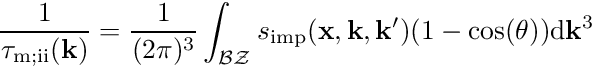
$\begin{align*} \lambda_{\mathrm D} = \frac{\epsilon k_{\mathrm{B}}T}{\mathrm{q}^2 (n+p)} \ . \end{align*}$

Similar to elastic acoustical phonon scattering, ionized impurity scattering does not couple different energy levels. However, a considerable complication stems from the angular dependence of the coefficient $\sigma_{\mathrm{imp}}$ . This complication can be circumvented by approximating the anisotropic coefficient by an elastic-isotropic process with the same momentum relaxation time $\tau_{\mathrm{m}; \mathrm{ii}}$ [11]. The momentum relaxation time is computed for an isotropic dispersion relation by an integration over the whole Brillouin zone and by weighting the change of direction of the momentum [14] :

$\begin{align*} \frac{1}{\tau_{\mathrm{m}; \mathrm{ii}}(\mathbf k)} = \frac{1}{(2\pi)^3} \int_{\mathcal{BZ}} s_{\mathrm{imp}}(\mathbf{x}, \mathbf{k}, \mathbf{k}^\prime) (1 - \cos(\theta)) \mathrm{d}\mathbf k^3 \end{align*}$

Here, the -axis for the integration in the Brillouin zone is chosen such that it is aligned with $\mathbf k$ , hence the angle between $\mathbf k$ and $\mathbf k^\prime$ is given by the inclination $\theta$ . Transformation to spherical coordinates leads to

$\begin{align*} \frac{1}{\tau_{\mathrm{m}; \mathrm{ii}}(\mathbf k)} = \frac{4\pi^3 N_{\mathrm I} \mathrm{q}^4}{\hbar\epsilon^2} \int_0^\infty \int_0^\pi \frac{1 - \cos(\theta)}{\left( 4 \vert \mathbf k \vert^2 \sin^2(\theta/2) + 1/\lambda_{\mathrm D}^2 \right)^2} \sin \theta \mathrm{d}\theta Z \mathrm{d}\varepsilon \end{align*}$

where the density of states is independent of the angles because of the assumption of an isotropic dispersion relation. The integral over the inclination $\theta$ can be computed analytically as

$\begin{align*} \int_0^\pi \frac{1 - \cos(\theta)}{\left( (\mathbf k^\prime - \mathbf k)^2 + 1/\lambda_{\mathrm D}^2 \right)^2} \sin \theta \mathrm{d}\theta = \frac{1}{4 \vert \mathbf k \vert^4} \left[ \ln(1+4 \lambda_{\mathrm D}^2 \vert \mathbf k \vert^2) - \frac{4 \lambda_{\mathrm D}^2 \vert \mathbf k \vert^2}{1+4 \lambda_{\mathrm D}^2 \vert \mathbf k \vert^2} \right] \ . \end{align*}$

Therefore, the isotropic scattering coefficient

$\begin{align*} s_{\mathrm{imp}; \mathrm{iso}}(\mathbf{x}, \mathbf{k}, \mathbf{k}^\prime) = \frac{\pi}{\hbar} \frac{N_{\mathrm I} \mathrm{q}^4}{\epsilon^2} \frac{1}{4 \vert \mathbf k \vert^4} \left[ \ln(1+4 \lambda_{\mathrm D}^2 \vert \mathbf k \vert^2) - \frac{4 \lambda_{\mathrm D}^2 \vert \mathbf k \vert^2}{1+4 \lambda_{\mathrm D}^2 \vert \mathbf k \vert^2} \right] \end{align*}$

has the same momentum relaxation time as the anisotropic coefficient given above. Note that $\vert \mathbf k \vert$ should be evaluated consistently with the approximated band. Moreover, since the Brooks-Herring model fails to correctly describe the carrier mobility at high doping concentrations, an empirical fit factor is usually employed in addition [11].

Impact Ionization Scattering

If free carriers acquire enough energy, they may lift electrons in the valence band to the conduction band after collision. This process is commonly referred to as impact ionization, where one electron generates an additional electron-hole pair. The final energy of an incoming electron with energy $\varepsilon$ is

$\begin{align*} \varepsilon^\prime = \frac{\varepsilon - E_{\mathrm{gap}}}{3} \ , \end{align*}$

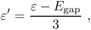
where it is assumed that all three carriers involved end up with the same kinetic energy. The impact ionization coefficient is typically modeled by a power-law with respect to the kinetic energy. Further details can be found in the textbook by Jungemann and Meinerzhagen [11].

Carrier-Carrier Scattering

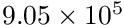
Very important for particularly the high energy tail of the distribution function is carrier-carrier scattering [19]. A carrier-carrier scattering mechanism requires that the two source states are occupied, and the two final states after scattering are empty. This leads to a scattering operator of the form

$\begin{align*} Q\{f\} = \frac{1}{(2\pi)^3} \int_{\mathcal{BZ}} \int_{\mathcal{BZ}} \int_{\mathcal{BZ}} & s(\mathbf{x}, \mathbf{k}^\prime, \mathbf{k}, \mathbf{k}_2^\prime, \mathbf{k}_2) f(\mathbf{x}, \mathbf{k}^\prime, t) (1-f(\mathbf{x}, \mathbf{k}, t)) f(\mathbf{x}, \mathbf{k}_2^\prime, t) (1-f(\mathbf{x}, \mathbf{k}_2, t))\\ & \ - s(\mathbf{x}, \mathbf{k}, \mathbf{k}^\prime, \mathbf{k}_2, \mathbf{k}_2^\prime) f(\mathbf{x}, \mathbf{k}, t)(1-f(\mathbf{x}, \mathbf{k}^\prime, t)) f(\mathbf{x}, \mathbf{k}_2, t)(1-f(\mathbf{x}, \mathbf{k}_2^\prime, t)) \mathrm{d}\mathbf k^\prime \mathrm{d}\mathbf k_2 \mathrm{d}\mathbf k_2^\prime \ , \end{align*}$

where the scattering coefficient $s(\cdot, \cdot, \cdot, \cdot, \cdot)$ now depends on the spatial location and on two pairs of initial and final states. With a low-density approximation, the nonlinearity of degree four of the carrier-carrier scattering operator reduces to second order:

$\begin{align*} Q_{\mathrm{cc}}\{f\} &= \frac{1}{(2\pi)^3} \int_{\mathcal{BZ}} \int_{\mathcal{BZ}} \int_{\mathcal{BZ}} s(\mathbf{x}, \mathbf{k}^\prime, \mathbf{k}, \mathbf{k}_2^\prime, \mathbf{k}_2) f(\mathbf{x}, \mathbf{k}^\prime, t) f(\mathbf{x}, \mathbf{k}_2^\prime, t) - s(\mathbf{x}, \mathbf{k}, \mathbf{k}^\prime, \mathbf{k}_2, \mathbf{k}_2^\prime) f(\mathbf{x}, \mathbf{k}, t) f(\mathbf{x}, \mathbf{k}_2, t) \mathrm{d}\mathbf k^\prime \mathrm{d}\mathbf k_2 \mathrm{d}\mathbf k_2^\prime \end{align*}$

The scattering coefficient can be derived to be of the form

$\begin{align*} s(\mathbf{x}, \mathbf{k}^\prime, \mathbf{k}, \mathbf{k}_2^\prime, \mathbf{k}_2) = \sigma_{\mathrm{cc}}(\mathbf x, \mathbf k, \mathbf k^\prime, \mathbf k_2, \mathbf k_2^\prime) \delta(\mathbf k + \mathbf k^\prime - \mathbf k_2 - \mathbf k_2^\prime) \delta(\varepsilon + \varepsilon^\prime - \varepsilon_2 - \varepsilon_2^\prime) \ , \end{align*}$

where the two delta distributions refer to conservation of momentum and energy respectively, and

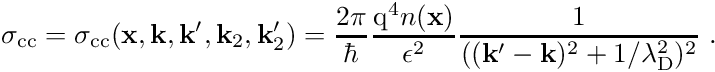
$\begin{align*} \sigma_{\mathrm{cc}} = \sigma_{\mathrm{cc}}(\mathbf x, \mathbf k, \mathbf k^\prime, \mathbf k_2, \mathbf k_2^\prime) = \frac{2\pi}{\hbar} \frac{\mathrm{q}^4 n(\mathbf x)}{\epsilon^2} \frac{1}{((\mathbf k^\prime - \mathbf k)^2 + 1/\lambda_{\mathrm D}^2)^2} \ . \end{align*}$

The set of parameters is similar to that of ionized impurity scattering, with the impurity density $N_{\mathrm a} + N_{\mathrm d}$ replaced by the carrier density . A projection onto spherical harmonics is very involved and is thus not further discussed here. Some details can be found in [22].

Boundary Conditions

As for any system of partial differential equations, the BTE needs to be equipped with boundary conditions in order to be completely specified. For the SHE method, different types of boundary conditions have been used.

In noncontact boundary regions, homogeneous Neumann boundary conditions with respect to the spatial coordinate are imposed. Similarly, homogeneous Neumann boundary conditions are imposed at the band-edge and at the highest energies considered in the simulation. At the contacts, ViennaSHE imposes either fixed Dirichlet conditions (Maxwellian distribution), or (by default) the recombination/generation-type boundary conditions as used by Schroeder et al. [24] and Jungemann et al. [3]. The refined boundary model proposed by Hong et al. [6] is not available in ViennaSHE yet.