This example is similar to mosfet.cpp, where a two-dimensional MOSFET simulation is carried out. This time, however, also quantum corrections as computed from the density gradient model are considered. A schematic of the considered device with segment numbers is as follows:
| Segment # | Segment description | Notes |
| 1 | Gate contact. | Potential known. |
| 2 | Source contact. | Potential known. |
| 3 | Oxide. | No boundary conditions, no carriers here. |
| 4 | Drain contact. | Potential known. |
| 5 | Source region. | n-doped region. |
| 6 | Body. | Intrinsic region. |
| 7 | Drain region. | n-doped region. |
| 8 | Bulk contact. | Potential known. |
| See Netgen geometry description in mosfet.in2d |
|
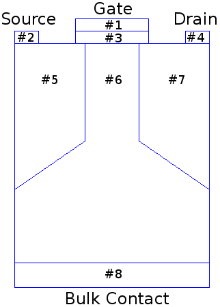
Schematic of the considered MOSFET
|
First Step: Initialize the Device
Once the device mesh is loaded, we need to initialize the various device segments (aka. submeshes) with material parameters, contact voltages, etc. For simplicity, we collect this initialization in a separate function:
template <typename DeviceType>
{
typedef typename DeviceType::segment_type SegmentType;
Provide convenience names for the various segments:
SegmentType const & gate_contact = device.segment(1);
SegmentType const & source_contact = device.segment(2);
SegmentType const & gate_oxide = device.segment(3);
SegmentType const & drain_contact = device.segment(4);
SegmentType const & source = device.segment(5);
SegmentType const & drain = device.segment(6);
SegmentType const & body = device.segment(7);
SegmentType const & body_contact = device.segment(8);
Now we are ready to set the material for each segment:
std::cout << "* init_device(): Setting materials..." << std::endl;
For all semiconductor cells we also need to specify a doping. If the doping is inhomogeneous, one usually wants to set this through some automated process (e.g. reading from file). For simplicitly we use a doping profile which is constant per segment. Note that the doping needs to be provided in SI units, i.e. 
std::cout << "* init_device(): Setting doping..." << std::endl;
device.set_doping_n(1e24, source);
device.set_doping_p(1e8, source);
device.set_doping_n(1e24, drain);
device.set_doping_p(1e8, drain);
device.set_doping_n(1e17, body);
device.set_doping_p(1e15, body);
Finally, we need to provide contact potentials for the device. Since we already have dedicated contact segments, all we need to do is to set the contact voltages per segment:
device.set_contact_potential(0.8, gate_contact);
device.set_contact_potential(0.0, source_contact);
device.set_contact_potential(0.1, drain_contact);
device.set_contact_potential(0.0, body_contact);
}
The main Simulation Flow
With the function init_device() in place, we are ready to code up the main application. For simplicity, this is directly implemented in the main() routine, but a user is free to move this to a separate function, to a class, or whatever other abstraction is appropriate.
First we define the device type including the topology to use. Here we select a ViennaGrid mesh consisting of triangles. See Application Programming Interface (API) or the ViennaGrid manual for other mesh types.
typedef DeviceType::segment_type SegmentType;
Read and Scale the Mesh
Since it is inconvenient to set up a big triangular mesh by hand, we load a mesh generated by Netgen. The spatial coordinates of the Netgen mesh are in nanometers, while ViennaSHE expects SI units (meter). Thus, we scale the mesh by a factor of  .
.
std::cout << "* main(): Creating and scaling device..." << std::endl;
DeviceType device;
device.load_mesh("../examples/data/mosfet840.mesh");
device.scale(1e-9);
Initialize the Device
Here we just need to call the initialization routine defined before:
std::cout << "* main(): Initializing device..." << std::endl;
Drift-Diffusion Simulations
In order to compute a reasonable initial guess of the electrostatic potential for SHE, we first solve the drift-diffusion model. For this we first need to set up a configuration object, and use this to create and run the simulator object.
std::cout << "* main(): Creating DD simulator..." << std::endl;
Prepare the Drift-Diffusion Simulator Configuration
In the next code snippet we set up the configuration for a bipolar drift-diffusion simulation. Although most of the options we set below are the default values anyway, we recommend the user to always set them manually in order to make the code more self-documenting.
Quantum Corrections: Enable the computation of quantum corrections via the density gradient model:
However, Do not use the correction potential in the continuity equations and just compute classic carrier concentrations. Here we just want to know the correction potential as a kind of error estimate.
Create and Run the DD-Simulator
With the config in place, we can create our simulator object. Note that after creating your simulator object, changes to the config will not affect the simulator object anymore. The simulator is then started using the member function .run()
std::cout << "* main(): Launching DD simulator..." << std::endl;
dd_simulator.run();
Write DD Simulation Output
Although one can access all the computed values directly from sources, for typical meshes this is way too tedious to do by hand. Thus, the recommended method for inspecting simulator output is by writing the computed values to a VTK file, where it can then be inspected by e.g. ParaView.
Calculate Terminal Currents
Since the terminal currents are not directly visible in the VTK files, we compute them directly here. To simplify matters, we only output the electron and hole drain currents from the body segment into the drain contact:
SegmentType const & drain_contact = device.segment(4);
SegmentType const & body = device.segment(6);
dd_simulator.potential(), dd_simulator.electron_density(),
body, drain_contact ) * 1e-6 << std::endl;
dd_simulator.potential(), dd_simulator.hole_density(),
body, drain_contact ) * 1e-6 << std::endl;
Self-Consistent SHE Simulations
To run self-consistent SHE simulations, we basically proceed as for the drift-diffusion case above, but have to explicitly select the SHE equations.
Similar to the case of the drift-diffusion simulation above, we first need to set up the configuration.
Prepare the SHE simulator configuration
First we set up a new configuration object, enable electrons and holes, and specify that we want to use SHE for electons, but only a simple continuity equation for holes:
std::cout << "* main(): Setting up first-order SHE (semi-self-consistent using 40 Gummel iterations)..." << std::endl;
Create and Run the SHE-Simulator
The SHE simulator object is created in the same manner as the DD simulation object. The additional step here is to explicitly set the initial guesses: Quantities computed from the drift-diffusion simulation are passed to the SHE simulator object by means of the member function set_initial_guess(). Then, the simulation is invoked using the member function run()
std::cout << "* main(): Computing first-order SHE..." << std::endl;
she_simulator.run();
Write SHE Simulation Output
With a spatially two-dimensional mesh, the result in (x, H)-space is three-dimensional. The solutions computed in this augmented space are written to a VTK file for inspection using e.g. ParaView:
std::cout << "* main(): Writing energy distribution function from first-order SHE result..." << std::endl;
she_simulator.config(),
she_simulator.quantities().electron_distribution_function(),
"mosfet-dg_she_edf");
Here we also write the potential and electron density to separate VTK files:
Write all macroscopic result quantities (carrier concentrations, density gradient corrections, etc.) to a single VTK file:
Calculate Terminal Currents
Since the terminal currents are not directly visible in the VTK files, we compute them directly here. To simplify matters, we only compute the electron current from the body segment into the drain contact based on the solution of the SHE equations:
device, config, she_simulator.quantities().electron_distribution_function(), body, drain_contact ) * 1e-6
<< std::endl;
Finally, print a small message to let the user know that everything succeeded
std::cout << "* main(): Results can now be viewed with your favorite VTK viewer (e.g. ParaView)." << std::endl;
std::cout << "* main(): Don't forget to scale the z-axis by about a factor of 1e12 when examining the distribution function." << std::endl;
std::cout << std::endl;
std::cout << "*********************************************************" << std::endl;
std::cout << "* ViennaSHE finished successfully *" << std::endl;
std::cout << "*********************************************************" << std::endl;
return EXIT_SUCCESS;
}
Full Example Code
#if defined(_MSC_VER)
#pragma warning(disable:4503)
#endif
#include <iostream>
#include <cstdlib>
#include <vector>
#include "viennagrid/config/default_configs.hpp"
template <typename DeviceType>
{
typedef typename DeviceType::segment_type SegmentType;
SegmentType const & gate_contact = device.segment(1);
SegmentType const & source_contact = device.segment(2);
SegmentType const & gate_oxide = device.segment(3);
SegmentType const & drain_contact = device.segment(4);
SegmentType const & source = device.segment(5);
SegmentType const & drain = device.segment(6);
SegmentType const & body = device.segment(7);
SegmentType const & body_contact = device.segment(8);
std::cout << "* init_device(): Setting materials..." << std::endl;
std::cout << "* init_device(): Setting doping..." << std::endl;
device.set_doping_n(1e24, source);
device.set_doping_p(1e8, source);
device.set_doping_n(1e24, drain);
device.set_doping_p(1e8, drain);
device.set_doping_n(1e17, body);
device.set_doping_p(1e15, body);
device.set_contact_potential(0.8, gate_contact);
device.set_contact_potential(0.0, source_contact);
device.set_contact_potential(0.1, drain_contact);
device.set_contact_potential(0.0, body_contact);
}
{
typedef DeviceType::segment_type SegmentType;
std::cout << "* main(): Creating and scaling device..." << std::endl;
DeviceType device;
device.load_mesh("../examples/data/mosfet840.mesh");
device.scale(1e-9);
std::cout << "* main(): Initializing device..." << std::endl;
std::cout << "* main(): Creating DD simulator..." << std::endl;
std::cout << "* main(): Launching DD simulator..." << std::endl;
dd_simulator.run();
SegmentType const & drain_contact = device.segment(4);
SegmentType const & body = device.segment(6);
dd_simulator.potential(), dd_simulator.electron_density(),
body, drain_contact ) * 1e-6 << std::endl;
dd_simulator.potential(), dd_simulator.hole_density(),
body, drain_contact ) * 1e-6 << std::endl;
std::cout << "* main(): Setting up first-order SHE (semi-self-consistent using 40 Gummel iterations)..." << std::endl;
std::cout << "* main(): Computing first-order SHE..." << std::endl;
she_simulator.run();
std::cout << "* main(): Writing energy distribution function from first-order SHE result..." << std::endl;
she_simulator.config(),
she_simulator.quantities().electron_distribution_function(),
"mosfet-dg_she_edf");
device, config, she_simulator.quantities().electron_distribution_function(), body, drain_contact ) * 1e-6
<< std::endl;
std::cout << "* main(): Results can now be viewed with your favorite VTK viewer (e.g. ParaView)." << std::endl;
std::cout << "* main(): Don't forget to scale the z-axis by about a factor of 1e12 when examining the distribution function." << std::endl;
std::cout << std::endl;
std::cout << "*********************************************************" << std::endl;
std::cout << "* ViennaSHE finished successfully *" << std::endl;
std::cout << "*********************************************************" << std::endl;
return EXIT_SUCCESS;
}


 1.8.7
1.8.7